
Abstract
Objective. Deep learning is increasingly permeating neuroscience, leading to a rise in signal-processing applications for extracellular recordings. These signals capture the activity of small neuronal populations, necessitating ‘spike sorting’ to assign action potentials (spikes) to their underlying neurons. With the rise in publications delving into new methodologies and techniques for deep learning-based spike sorting, it is crucial to synthesise these findings critically. This survey provides an in-depth evaluation of the approaches, methodologies and outcomes presented in recent articles, shedding light on the current state-of-the-art. Approach. Twenty-four articles published until December 2023 on deep learning-based spike sorting have been examined. The proposed methods are divided into three sub-problems of spike sorting: spike detection, feature extraction and classification. Moreover, integrated systems, i.e. models that detect spikes and extract features or do classification within a single network, are included. Main results. Although most algorithms have been developed for single-channel recordings, models utilising multi-channel data have already shown promising results, with efficient hardware implementations running quantised models on application-specific integrated circuits and field programmable gate arrays. Convolutional neural networks have been used extensively for spike detection and classification as the data can be processed spatiotemporally while maintaining low-parameter models and increasing generalisation and efficiency. Autoencoders have been mainly utilised for dimensionality reduction, enabling subsequent clustering with standard methods. Also, integrated systems have shown great potential in solving the spike sorting problem from end to end. Significance. This survey explores recent articles on deep learning-based spike sorting and highlights the capabilities of deep neural networks in overcoming associated challenges, but also highlights potential biases of certain models. Serving as a resource for both newcomers and seasoned researchers in the field, this work provides insights into the latest advancements and may inspire future model development.

Original content from this work may be used under the terms of the Creative Commons Attribution 4.0 license. Any further distribution of this work must maintain attribution to the author(s) and the title of the work, journal citation and DOI.
1. Introduction
Neurons communicate through the exchange of electrical impulses, more precisely, through the release of neurotransmitters, which results in the propagation of action potentials [1]. Signals of individual neurons and the signal exchange with their neighbours are usually investigated with extracellular recordings. Extracellular electrodes typically capture the activity of a small group of neurons. According to an approximation by Pedreira et al [2], which is based on the assumption that there are 300 000 neurons mm3 (as in the rat hippocampus [3]), following Coulomb’s law for amplitude decay as v∼1/r2, and assuming that action potentials of ∼60 µV are generated at a distance of 50 µm [4] (maximum distance and minimum amplitude to identify single spikes), more than thirty neurons would generate spikes with an amplitude ranging from 60 µV to 70 µV, and around ten neurons would generate amplitudes between 100 µV and 110 µV. However, the measured signals are contaminated by noise originating from neurons not close to the electrode. Additionally, artefacts originating from the recording equipment influence the recorded signal, resulting in fewer spikes reaching the above voltage levels. Neuronal waveforms exhibit distinct characteristics, primarily determined by the cell type, ion channel distribution, dendritic tree morphology, and the orientation and distance to the recording electrode [5, 6]. These features enable spike sorting, i.e. extracting spikes from neural recordings and assigning them to their underlying neurons. Multi-electrode arrays (MEA), such as tetrodes or polytrodes, enable the utilisation of spatial spike features, e.g. by triangulation [4]. High-density MEA (HD-MEA) recordings with hundreds of channels are already in use [7] and with the growing number of neurons being measured, it has become imperative to employ automatic, high-bandwidth spike sorting algorithms to analyse single neuron activity at scale. Advancements in spike sorting and HD-MEA technologies are essential for neuroscience research, clinical applications, and brain–computer interfaces (BCIs). In fundamental neuroscience, spike sorting offers valuable insights into the functioning of neuronal circuits, advancing our understanding of the interactions between cerebral regions and behaviours. Clinically, the analysis of extracellular recordings is vital for studying neurological conditions, including epilepsy [8], paralysis [8, 9], and cognitive loss [10]. Spike sorting is also crucial for neural signal decoding and their translation into commands for external device control in BCIs and neuroprosthetics [5]. It has been shown that single-neuron activity can help to decode movement [8], intentions [11], and memory [10].
Deep neural networks (DNNs) are becoming increasingly important in neuroscience. In neuroimaging, deep learning is used to detect and analyse Alzheimer’s disease [12], brain strokes [13], autism [14], and other neurological and psychiatric disorders [15]. Deep learning models enhance neuroimaging techniques by automating the segmentation of brain images, for example, to detect brain tumors [16] or improve signal extraction from noisy data [17]. Also, deep learning is used to model neurodegenerative diseases and analyse their underlying mechanisms [18]. Other deep learning applications in neuroscience research include decoding brain activity on a macro level, e.g. by analysing functional magnetic resonance images [19] or electroencephalogram (EEG) [20], and on a micro level, by analysing intracranial micro-electrode recordings, e.g. for spike sorting [21]. For the latter, deep learning offers the potential to handle high-dimensional data, perform automatic feature learning, and improve system scalability and noise robustness. For decades, attempts have been made to solve the spike sorting problem, and many reviews have tried to provide insights on the state-of-the-art [4, 22–25]. Recent reviews on spike sorting methods [26–29] do not consider DNN-based models in detail. To address this gap, this survey provides a comprehensive evaluation of current approaches on deep learning-based spike sorting.
The first section of this paper provides a brief overview of conventional spike sorting methods and different types of data commonly used for their evaluation. Also, the challenges of spike sorting and requirements for modern spike sorting algorithms are outlined. Section 2 focuses on state-of-the-art spike sorting methods that are not based on neural networks (NNs), followed by brief historical developments related to the application of NNs in spike sorting. Subsequently, two innovative studies are examined to demonstrate that NNs with a single hidden layer can be used in various spike sorting scenarios, showcasing both the limits and advantages of such shallow models. The criteria for the selected publications in this survey are also outlined. Section 3 focuses on spike detection, section 4 deals with feature extraction, section 5 covers classification models, and section 6 focuses on integrated systems, i.e. DNNs that detect spikes and perform feature extraction or classification using a single model. Section 7 critically discusses how state-of-the-art deep learning-based spike sorting models address the challenges and requirements described in section 1.3, identifies future directions and outlines hardware implementations of certain models. Concluding remarks are drawn in section 8.
1.1. Conventional spike sorting
Traditionally, the spike sorting procedure is separated into several steps, as shown in figure 1. Using a band-pass filter on the raw data, the signal of interest consisting of neural activities can be isolated. Single spikes can be detected with techniques like adaptive amplitude or power thresholding. As these methods may lead to inclusions of non-neural activity (false-positives) and spikes still can be missed (false-negatives), other techniques, such as the non-linear energy operator [30] or the continuous wavelet transformation [31], have been applied extensively to detect spikes. Once detected, spikes are typically aligned to their amplitude peaks for subsequent analysis [24], and features are extracted in order to reduce dimensions. Standard feature extraction methods include principal component analysis (PCA) [32], independent component analysis [33], t-distributed stochastic neighbour embedding (t-SNE) [34], and discrete wavelet transform [35]. Subsequently, the extracted spike features are clustered, often using the k-means algorithm [36], where each centroid represents a template for a particular neuron. While k-means requires k as a parameter for the number of clusters in the data, density-based spatial clustering of applications with noise (DBSCAN) [37] does not require information about the number of clusters but often fails to identify clusters of varying density and requires careful hyperparameter tuning. Hierarchical [38] and Bayesian clustering [39] are also frequently used to cluster neural data. Spike trains, i.e. binary signals that indicate the temporal firings of a single neuron, are the desired outcome of spike sorting and are generated with the obtained spike times for each cluster. The explained pipeline represents unsupervised spike sorting, where data patterns and similarities within the data are identified to group similar spike waveforms. However, supervised learning is increasingly being used in machine learning-based spike sorting, where support vector machines [40] and NNs [41, 42] trained with labelled data can be used for both spike detection and classification, effectively mapping spikes to their underlying neurons.
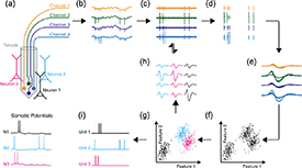
Figure 1. Conventional pipeline for unsupervised spike sorting. (a) Four electrodes capture changes in the electrical activity of three neurons near to the electrode. The raw data (b) typically are processed with a band-pass filter (c), which enables spike detection (d). Subsequently, the spikes are aligned (e) to extract features (f). Clustering can be applied to the low level feature space to group the spiking events (g), where the average of one cluster is called template (h). Finally, the spike trains can be reconstructed with the corresponding spike times (i). With permission from [23]. Reprinted from [23], Copyright (2011), with permission from Elsevier.
Download figure:
Standard image High-resolution image1.2. Datasets
Three types of datasets are commonly used to evaluate spike sorting algorithms: (i) real extracellular recordings, (ii) synthetic datasets, and iii) hybrid datasets. Among these datasets, real extracellular recordings are the most challenging, as they encapsulate a myriad of real-world challenges, such as artefacts or multi-component noise, rendering them intricate but invaluable for advanced analyses. A significant limitation of real data is the absence of ground truth (GT). Patch clamp recordings [43] are frequently employed in this particular setting due to their capability to offer a precise and direct assessment of neuronal activity, thus serving as a dependable reference point. However, they require a significantly greater effort in recording. Thus, synthetic datasets have ascended as a standard for evaluation. Synthetic data are meticulously constructed and typically mimic a local field potential (LFP), often generated by numerous overlapping spike templates, upon which various spike templates are subsequently superimposed at a larger scale to emulate the activity of a small number of neurons in the vicinity of the electrode [44]. Despite their utility, synthetic datasets have inherent limitations, as they often lack the incorporation of practical scenarios such as bursting neurons, electrode drift, or transient noise. To address these gaps, hybrid datasets have been employed frequently, combining the strengths of real and synthetic data for more accurate analysis and interpretation. Various platforms, such as Collaborative Research in Computational Neuroscience [45], SpikeForest [46], or individual labs with public data repositories [47, 48] provide access to large data from several species and brain regions acquired with various electrode types.
1.3. Challenges and requirements
Transient signals are one of the biggest challenges in spike sorting, as the recorded noise level may fluctuate [49], and spike waveforms often vary in their expression [5, 6]. Since the neuron-electrode distance and orientation can change during a recording, the measured voltages may vary over time, resulting in electrode drift [24]. Moreover, neurons exhibit burst firing patterns, leading to an amplitude decrease of up to 80% [4]. In 2012, Pedreira et al discussed several reasons why the amount of identified neurons per channel appeared lower than expected with existing spike sorters, pointing to sparsely firing neurons as one possible reason [2]. Such neurons pose a significant challenge, especially for template-matching approaches, as they require a specific template for each firing neuron. This, along with transient waveforms, makes adaptive algorithms necessary. Since each channel in an extracellular recording captures the activity of several neurons, two or more neurons may fire simultaneously, leading to overlapping waveforms in the recording. Spike overlaps have been studied for decades and yet have not been fully resolved [50–52]. Moreover, spike sorting models are usually subject to the missing ground-truth problem, as the number of firing neurons during a recording is typically unknown in real-world situations. Furthermore, modern spike sorting models must be scalable to handle HD-MEA recordings. Resource-efficient data processing methods are therefore required for hardware implementation without jeopardising online processing. Implantable on-chip processors for spike sorting are particularly advantageous because they can massively reduce the data rate to be transferred, which directly impacts the power consumption of resource-limited brain chips. On-chip compression models are an alternative approach to reduce the data that needs to be transferred. Apart from that, robust spike sorting algorithms must be transferable for use on different subjects, brain areas, and electrode types. Given the practical limitations, the capacity to generalise across various setups is not just convenient but essential. Reproducibility is another requirement of modern algorithms. Spike sorting models often involve many hyperparameters that require careful tuning for optimal performance. In order to accelerate collaborative progress, it is therefore important that new models (code and data repositories) are published open access.
2. Background and literature overview
2.1. State-of-the-art spike sorting
Superparamagnetic clustering (SPC) was introduced to spike sorting by Quiroga et al in 2004 [44] and is still used as a benchmark. In SPC, data are grouped by evaluating spin–spin correlations derived from the ferromagnetic model of the data. SPC sorts spikes in an unsupervised fashion and provides high accuracy at the expense of computation. Osort [53], one of the first advanced spike sorting algorithms for online processing, is another method that does not require knowledge of the number of clusters in the data. Other online sorting algorithms include GEMsort [54], an on-implant sorter that is based on salient feature selection [55] and Geo-OSort [56] which are mentioned here to increase the technical depth of this survey. Recent advancements in HD-MEA have increased the signal quality, leading to a rise in detectable action potentials with more overlapping spikes [57]. As a result, source separation models have emerged as the preferred approach to process multi-channel recordings. Kilosort [21], one such model, processes neural data in several stages, including pre-processing, clustering, template-matching and post-processing. Kilosort employs a modified k-means clustering technique that is robust to amplitude alterations in spikes. This improves its robustness and flexibility in handling different signal fluctuations, thus enhancing its performance in spike sorting tasks. In 2024, Pachitariu et al proposed Kilosort4, which could improve the clustering stage using a graph-based approach [58]. Kilosort4 is recognised for its ability to accurately detect neurons with low amplitudes and small spatial extents, even under conditions of high drift, which is essential to accurately identify neuronal spikes in challenging recording conditions [58]. Despite the advantages of Kilosort, there are also limitations, which may be affected by various factors, including electrode density, signal-to-noise ratio (SNR) and computational resources, potentially providing suboptimal results in specific conditions. Furthermore, the Kilosort algorithm has tuneable parameters. Although good results can be achieved with the default settings, adjusting the parameters can introduce bias. In 2017, MountainSort [59], another advanced spike sorting system for HD-MEA data, was introduced by Chung et al. MountainSort has also been iteratively improved since its introduction, leading to the recent release of MountainSort4 [60], an efficient spike sorting algorithm that first over-clusters spikes based on the geometric layout of the electrode array and then merges clusters across adjacent channels to remove redundancy. One of its main benefits is its model independence, enabling it to efficiently manage variations in non-Gaussian waveforms under various recording conditions [59]. Compared to Kilosort, this algorithm is fully automatic at the expense of accuracy. Other popular algorithms reported in recent years are KlustaKwik [61], SpyKING CIRCUS [62], and IronClust [63]. Recently, Pachitariu et al reported that IronClust is the nearest competing algorithm to Kilosort4, especially under electrode drift. At the same time, SpyKING CIRCUS and MountainSort4 performed similarly to IronClust on non-drifting recordings [64]. Although Kilosort4 is perhaps one of the best contemporary solutions, there is still scope for improvement; e.g. fast electrode drift still poses a problem [64].
2.2. Spike sorting with NNs
NN-based spike sorting dates back to 1988, when Bower et al used a Hopfield network to associate memory with binary thresholds for spike classification [65]. While the 1990s saw advancements with single-hidden-layer NNs (SHL-NNs) for spike detection and classification [66–68], the field continued to evolve, leading to the exploration of self-organising maps [69–71], known for their unsupervised learning capabilities. The quest for computational efficiency in spike sorting led to the emergence of spiking NNs (SNNs) [72–75], which mirror the time-dependent nature of biological NNs more closely. Running on neuromorphic hardware, SNNs can exploit their full potential, offering benefits in terms of energy efficiency due to sparse, event-driven computations and the ability to recognise spatiotemporal data patterns [76], but often depend on precise hyperparameter tuning [27].
Several SHL-NNs targeting specific tasks in the spike-sorting pipeline have been proposed recently. In the following, two such solutions are briefly described. In 2020, Issar et al [41] proposed a multi-layer perceptron (MLP) to separate spikes from noise that impaired decoding. A supervised learning model was developed to predict the probability that a given waveform is a spike [41]. The model was trained with 24 810 795 labelled waveforms derived from extracellular recordings from four monkeys, two brain regions, two recording devices and different implant ages [41]. Qualitatively, the network’s spike classifications from two additional subjects were consistent with human expert classifications; quantitatively, the model improved the decoding accuracy compared to traditional threshold-crossing methods [41]. However, the model struggled with diverse spikes from different brain regions and recording devices. Here, a deep model could be helpful to increase performance. According to early theoretical findings by Cybenko [77], a network equipped with a single hidden layer comprising sigmoid units can effectively approximate any decision boundary if the layer is large enough. However, to avoid an impractically large hidden layer, it is advisable to use deep models. The hierarchical structure of DNNs enables capturing both low-level and high-level features, making them particularly adept at handling variable spikes, superpositions and transient noise. In 2021, Valencia and Alimohammad [42] developed a binarised NN (BNN) for spike classification. In a BNN, weights and activations are binarised to reduce the required memory and computational load. In [42], the BNN takes previously detected and aligned spikes and classifies them according to their underlying neuron. With their SHL-BNN, Valencia and Alimohammad reached an average classification accuracy of 90% on the widely used synthetic dataset that was initially presented in [44]. In sections 4 and 5, it will be seen that full-precision DNNs [78] can achieve an accuracy of more than 99% on the same data, by also using supervised learning schemes. However, the model type and architecture always determine a trade-off between efficiency and effectiveness. In this paper, DNNs refer to models with more than one hidden layer. MLPs, convolutional NNs (CNNs), recurrent NNs (RNNs), especially long short-term memory (LSTM) networks, autoencoders (AEs), and generative adversarial networks (GANs) are the focus of this work.
2.3. Literature overview
The literature was screened using the databases of PubMed and Google Scholar. The following keywords were used for the search: (‘Spike Sorting’ OR ‘Spike Detection’ OR ‘Spike Classification’) AND (‘NN*’ OR ‘Deep Learning’ OR ‘MLP’ OR ‘MLP’ OR ‘CNN*’ OR ‘ConvNet*’ OR ‘CNN’ OR ‘RNN*’ OR ‘RNN’ OR ‘LSTM’ OR ‘LSTM’ OR ‘AE*’). Due to the large number of publications found, several criteria were defined to narrow the focus this study. The core subjects of this work are deep learning-based spike detection, feature extraction and classification for extracellular recordings of the brain. Only articles that fulfil the following criteria were considered:
- Published until December 2023.
- Peer-reviewed.
- The model presented in the respective article;
- has a deep architecture,
- was evaluated using extracellular recordings,
- is not a denoising or compression model,
- is not based on reinforcement learning,
- is not an SNN or neuromorphic model,
- is not a spike sorting post-processor.
After all relevant literature was gathered, the references of all collected papers were screened to find additional articles within the scope of this survey. Table 1 provides an overview of twenty-four publications considered in this work. Entries in table 1 between two columns indicate that the respective model was used for both tasks in the spike sorting pipeline. As deep classification networks perform feature extraction in the hidden layers of the model, these models are always situated between the ‘feature extraction’ and ‘clussification/clustering’ column in table 1. Figure 2 illustrates the breakdown of the different network types utilised in the examined studies. For clarity, classification networks are not represented as feature extractors in figure 2.

Figure 2. Treemap of the deep learning model types used in all considered studies. Note that AE architectures in table 1 and this illustration often contain convolutional or LSTM layers, and CNNs usually contain dense layers at the output.
Download figure:
Standard image High-resolution imageTable 1. Recently developed spike sorting solutions using deep learning-based models in chronological order. Models that are publicly available are highlighted in bold.
| References | Authors | Datasets | Channel type | Detection | Feature extraction | Classification/ clustering | Significance of the deep learning-based approach |
|---|---|---|---|---|---|---|---|
| [79] | Lee et al | [80, 81] | Single | CNN | PCA | Gaussian Mixture Model | Detection of neural spikes with improved spatiotemporal alignment. |
| [82] | Yang et al | [44, 83] | Single | Peak detection | PCANet | SVM | Low complexity sorting with similar accuracy to conventional methods. |
| [84] | Wu et al | [44, 84] | Single | Median-based | GAN | Few-shot sorting enabled by semi-supervised adversarial representation learning. | |
| [85] | Saif-ur-Rehman et al | [85–87] | Single | CNN | — | — | Universal neural channel tracking that works across species, brain regions & electrodes. |
| [88] | Rácz et al | [89] | Multi | CNN + LSTM | CNN | Spatiotemporal spike classification using HD-MEA data (128 channels). | |
| [78] | Park et al | [2, 44, 90] | Single | Thresholding | MLP | Improved accuracy and runtime compared to standard methods like PCA + k-means. | |
| [91] | Wouters et al | [92] | Multi | — | MLP | k-means | Resolved overlapping spikes in the feature space using a custom cost function. |
| [93] | Markanday et al | [93] | Single | CNN | — | — | Human expert-level detection of complex spikes produced by cerebellar Purkinje cells. |
| [94] | Ciecierski | [95] | Single | — | GAN | Unsupervised spike sorting with a GAN, using a ‘spike-aware’ loss function. | |
| [96] | Eom et al | [2, 44, 90, 97] | Multi | Thresholding | AE | DBSCAN | Unsupervised feature extraction by combining latent space representations of three AEs. |
| [98] | Li et al | [44, 99] | Single | — | CNN | Improved spike classification accuracy due to many convolutional layers. | |
| [100] | Saif-ur-Rehman et al | [44, 85–87] | Single | CNN + CNN | PCA | k-means | Background activity rejection reduces the number of waveforms for subsequent analysis. |
| [101] | Rokai et al | [46, 89, 102] | Multi | AE | Integrated model for online spike detection and classification using HD-MEA data. | ||
| [103] | Seong et al | [44, 104] | Single | Thresholding | AE | k-means | Unsupervised feature extraction utilising a quantised model; implemented on an ASIC. |
| [105] | Yi et al | [2, 105] | Multi | MountainSort | CNN | Spike classification with a quantised model, using HD-MEA data; FPGA implemented. | |
| [106] | Liu et al | [44, 99] | Single | — | CNN + LSTM | Optimised classification of overlapping spikes by combining CNN and LSTM. | |
| [107] | Radmanesh et al | [43, 45, 108] | Single | — | AE | SVM | Noise-robust unsupervised feature extraction using a deep contractive AE. |
| [109] | Okreghe et al | [44, 86, 87, 110] | Multi | CNN + CNN | PCA | k-means | Improved channel selection and artefact removal using spatiotemporal spike data. |
| [111] | Ardelean et al | [2, 111] | Single | Thresholding | AE | k-means | Network complexity has to be designed relatively to the complexity in the neural data. |
| [112] | Rokai et al | [43, 46, 62] | Multi | CNN | Isosplit5 | Input-source agnostic spike detection and feature embedding using edgeTPU hardware. | |
| [113] | Wang et al | [44, 75, 99, 114] | Single | CNN + CNN | CNN + LSTM | Spike detection and localisation with 2 CNNs and sorting with a sliding-window LSTM. | |
| [115] | Zhang et al | [44] | Single | — | CNN | CNN taking Log-Mel spectrogram as input to classify overlapping spikes. | |
| [116] | Meyer et al | [44, 99] | Single | MLP | Lightweight detection and sorting with downstream validation to enhance performance. | ||
| [117] | Zacharelos et al | [108] | Single | MLP | Lightweight detection and sorting; ASIC implemented, using approximate computing. | ||
3. Spike detection
In this section, the focus is on DNN-based spike detection models. The models’ practical relevance is elucidated, highlighting their strengths and weaknesses and comparing them when feasible. In 2017, Lee et al [79] presented a CNN to detect neural spikes; it is part of the well-known spike sorting algorithm called YASS [79]. The first layers in CNNs are known to capture basic features of the input, e.g., edges in images, while deeper layers capture more complex features, e.g. specific objects in images. A relatively small number of kernels (filters, or weights and biases) are applied to the input with a specified stride, which reduces the chances of overfitting and helps to concentrate on specific patterns, regardless of their position in the input. The CNN in [79] takes data from a single channel, propagates it through two hidden layers and returns binary labels (‘spike’ or ‘no spike’). Lee et al used the rectified linear unit (ReLU) activation function,  if
 , else
 , to add non-linearity to the system [79]. Moreover, L2 regularisation, also known as weight decay, was applied to prevent overfitting. Tested on various noise levels, the proposed CNN outperformed several contemporary detection techniques [79]. In 2020, a further developed model of YASS was published [118], still using a CNN for spike detection, but processing multi-channel data. Note that [118] has not been peer-reviewed. As in [79], data augmentation was utilised to create a training set based on pre-sorted spikes with artificial overlaps at random scales and shifts [118]. Temporal and spatial filters were segregated to enhance network speed, with the initial layer focusing to extract temporal characteristics and the subsequent layer capturing features from adjacent spatial channels [118]. Lee et al tailored their model to retina recordings, where overlapping spikes occur frequently. 70% of the positive events in the generated training data consisted of spike collisions [118]. YASS [118] consists of the following sub-algorithms: spike detection, denoising, de-duplication, spike division for parallel processing, clustering by using iterative featurisation, triaging and deconvolution. A clear advantage of such a procedural pipeline is that the CNN could be easily replaced with other detection models. The performance of YASS [118] was compared with other state-of-the-art sorters like Kilosort [21], SpyKING CIRCUS [62] and MountainSort [59], where Kilosort achieved the highest performance. YASS was significantly better than Kilosort at restoring spikes on retinal ganglion cell types, as the CNN in [118] was trained especially on retinal recordings. To avoid a potential bias in their evaluation, Lee et al [118] tested their model using a second hybrid dataset, where YASS performed best. The CNN contributes by finding many spikes missed by other sorters and improving spatiotemporal alignment [79].
In 2019, Rácz et al [88] proposed a convolutional LSTM network to detect spikes in HD-MEA data. An LSTM network represents a form of RNN that addresses the intricacies of sequence prediction problems. During a forward pass, it takes a series of inputs and processes each element by maintaining a cell state and a hidden state throughout the sequence. An integral part of its functionality lies in implementing distinctive gating mechanisms, namely the forget, input, and output gates, acting as guardians governing the flow of information. LSTM networks have the ability to capture long-term dependencies within the data through the coordinated interplay of these gates. In [88], recordings from 128 channels arranged in a 32 × 4 grid were applied to an LSTM network. Table 2 details the model architecture employed in [88] including the type of each layer, data dimensions (Dim.), kernel sizes, and strides. Convolutional layer dimensions are denoted as ‘number of filters @ dimensions’. The network was trained using pseudo-labels obtained by Kilosort [21]. For regularisation [88], used an early stopping criterion that terminates model training if the loss of the system does not decrease for a specified number of epochs. Another regularisation technique used in [88] that also speeds up training is batch normalisation [119], which forces the layer inputs to have a mean of zero and a standard deviation of one. Rácz et al utilised nine 45 min recordings, using 90% of the data for training and the remaining 10% for testing. Ten positive predictions were considered as spikes for evaluation [88]. It should be noted that the results of the model in [88] were evaluated in relation to Kilosort’s performance, which does not make the achieved results entirely conclusive. However, this is often the case for models that were evaluated using real-world data. The DNN in [88] yielded a true positive rate (also called recall or sensitivity) of around 70% and a precision (accuracy of the model in classifying a sample as positive) of only 19%. In this regard, Rácz et al concluded that low precision should not lead to trouble for sophisticated sorters as they may discard false positives [88]. Nevertheless, this leads to redundant data processing of noisy segments. Furthermore, a recall of 70% still implies a lot of false negatives, making the model in [88] unsuitable for practical use despite extensive training and a sophisticated architecture.
Table 2. Model architecture of the CNN-LSTM in [88].
| # | Type | Dim. | Kernel | Stride |
|---|---|---|---|---|
| 0 | Input | 32 × 4 | — | — |
| 1 | 2D-Conv | 16 @ 28 × 3 | 5 × 2 | 1 × 1 |
| 2 | 2D-Conv | 256 @ 24 × 2 | 5 × 2 | 1 × 1 |
| 3 | Pooling | 256 @ 12 | 2 × 2 | 2 × 2 |
| 4 | LSTM | 512 | — | — |
| 5 | Dense | 512 | — | — |
| 6 | Dense | 256 | — | — |
| 7 | Dense | 2 | — | — |
In 2023, Wang et al [113] proposed a method for spike detection working with single-channel data that is based on a two-stage procedure involving two CNNs. Firstly, the continuous single-channel signal was divided into sliding windows of 200 samples, using an overlap of 20%. This segmented data was then applied to a CNN that predicts the input as neural or background activity. The architecture of the CNN in [113] is described in table 3, where σ(x) denotes the used activation functions. Note that missing entries for both dense layers do not necessarily imply that no activation function was used but mean that it was not mentioned in the respective paper. As can be seen in table 3, the Softmax activation function,  , where i represents the index of the current class and j denotes the indices over all classes, was utilised to determine probabilities for both classes (‘spike’ or ‘no spike’). In the second stage, spikes were localised within the 200 sample-long signal snippets. The architecture of this model is identical to the one described in table 3, but skips the first convolutional layer. Moreover, this model’s final layer predicts the spikes’ start and end positions [113]. Both CNNs were trained with labelled data and compared against different network architectures, e.g. LSTM, with the proposed CNN showing the best performance [113]. Experiments with varying noise levels showed that this factor directly influenced the detection quality. However, it is assumed that this is the case for most models presented in this survey, as high noise aggravates distinguishing spikes from artefacts. Irrespective of this, using sliding windows for spike detection ensures that any spike signal intercepted by a window slice will still be captured within the subsequent window, but also introduces redundant data processing. The CNN in [113] is limited to detecting one spike at a time. For practical applications, it is therefore essential to expand this model into a multi-target detector.
Table 3. Model architecture of the CNN in [113].
| # | Type | Dim. | σ(x) | Kernel | Stride |
|---|---|---|---|---|---|
| 0 | Input | 200 | — | — | — |
| 1 | 1D-Conv | 20 @ 200 | ReLU | 3 | 1 |
| 2 | Pooling | 20 @ 50 | — | 4 | 4 |
| 3 | 1D-Conv | 50 @ 50 | ReLU | 3 | 1 |
| 4 | Pooling | 50 @ 12 | — | 4 | 4 |
| 5 | Dense | 550 | — | — | — |
| 6 | Dense | 200 | — | — | — |
| 7 | Dense | 2 | Softmax | — | — |
3.1. Neural channel selection and artefact removal
In 2019, Saif-ur-Rehman et al proposed Spikedeeptector [85], a CNN designed to detect and track channels containing neural data. This is helpful in identifying useful channels for BCI applications [85]. The proposed CNN is a supervised learning model and relies, like the models described above, on the quality of labelled training data. Saif-ur-Rehman et al used a semi-automatic method to acquire pseudo-labels, including visual inspections [85]. The training data was taken from a single subject (1.56 million feature vectors that are batches of waveforms from a single channel with a size of 48 × 20 samples). If at least one of these waveforms represented a spike, the whole batch was classified as neural. The CNN applied for this task is detailed in table 4. While the first layer performs a convolution through time, the second layer convolves over the entire batch. For training, the authors used L2-regularisation, early stopping, batch normalisation and dropout [120] as regularisation techniques to improve generalisation. Dropout is a simple yet effective technique to prevent overfitting by randomly ignoring selected units during training, preventing certain co-adaptations on the training data. As the CNN in [85] only assigns labels to a given feature vector, Saif-ur-Rehman introduced a criterion that calculates the mode of the predicted outputs to classify entire channels as ‘neural’ or ‘noisy’. Overall, an accuracy of 97.2% could be achieved with Spikedeeptector [85]. Notably, the model could generalise across different brain regions, subjects, species and electrode types. Spikedeeptector may be used to identify and exclude threshold-crossing artefacts from subsequent analysis. However, complex artefacts can still affect the model as these events may occasionally be classified as neural. In a follow-up study published in 2021 [100], Saif-ur-Rehman et al developed an additional CNN called ‘background activity rejector’ (BAR) that takes signals selected by Spikedeeptector and discards background activity by classifying a given signal as spike or noise [100]. The architecture of BAR is detailed in table 5. This model also utilises batch normalisation and L2 regularisation to prevent overfitting. Labelled data of two species, five subjects, six brain areas, three different types of electrodes and two recording systems were used for training to create a robust system [100]. Evaluated on data from three human subjects, BAR could achieve an accuracy of 92.3%. Further considerations regarding the scalability of this model can be found in section 7.1.
Table 4. Model architecture of Spikedeeptector [85].
| # | Type | Dim. | σ(x) | Kernel | Stride |
|---|---|---|---|---|---|
| 0 | Input | 48 × 20 | — | — | — |
| 1 | 2D-Conv | 25 @ 48 × 20 | ReLU | 3 × 1 | 1 × 1 |
| 2 | 2D-Conv | 25 @ 46 | ReLU | 3 × 20 | 1 × 1 |
| 3 | Pooling | 25 @ 23 | — | 2 × 1 | 1 × 1 |
| 4 | 2D-Conv | 50 @ 21 | ReLU | 3 × 1 | 1 × 1 |
| 5 | Pooling | 50 @ 11 | — | 2 × 1 | 1 × 1 |
| 6 | 2D-Conv | 100 @ 9 | ReLU | 3 × 1 | 1 × 1 |
| 7 | Pooling | 100 @ 5 | — | 2 × 1 | 1 × 1 |
| 8 | Dense | 100 | ReLU | — | — |
| 9 | Dense | 2 | Softmax | — | — |
Table 5. Model architecture of BAR [100].
| # | Type | Dim. | σ(x) | Kernel | Stride |
|---|---|---|---|---|---|
| 0 | Input | 48 | — | — | — |
| 1 | 1D-Conv | 25 @ 48 | ReLU | 3 | 1 |
| 2 | 1D-Conv | 50 @ 44 | ReLU | 5 | 1 |
| 3 | Pooling | 50 @ 22 | — | 2 | 1 |
| 4 | 1D-Conv | 50 @ 18 | ReLU | 5 | 1 |
| 5 | Pooling | 50 @ 9 | — | 2 | 1 |
| 6 | Dense | 50 | ReLU | — | — |
| 7 | Dense | 2 | Softmax | — | — |
In 2023, Okreghe et al [109] also worked on a solution for improved channel selection and artefact removal. The basic approaches of Saif-ur-Rehman et al [100] and Okreghe et al [109] are similar and illustrated in figure 3. The method in [109], called ‘deep spike detection’ (DSD), also works with two CNNs: one for the selection of channels and one for artefact removal. Like the work above, DSD was trained with many labelled feature vectors (1.61 million) to create a robust network. Contrary to the work of Saif-ur-Rehman et al [85], the authors of [109] applied Kilosort [21] to obtain pseudo-labels. Moreover, instead of taking twenty waveforms from a single channel, they used waveforms from multiple channels as an input for DSD to utilise spatiotemporal data dependencies, similar to [88, 118]. The first CNN has the same architecture as Spikedeeptector (table 4). As in [85], a batch (48 × 20) was labelled as ‘neural’ if it contained at least one spike waveform [109]. Naturally, a larger batch size increases inference time, which may affect online processing, but also yields better results (99.62% for a batch size of 100; 97.51% for a batch size of 20). Like BAR [100], the second CNN (artefact removal network) is provided with a single feature vector (48 × 1) and discards non-neural events [109]. The architecture of this CNN also resembles BAR, which was presented in [100] (table 5). Using the data in [109], the artefact removal network could achieve an overall accuracy of 92.3%. Using both simulated and experimental datasets, integrating DSD into a traditional spike sorting pipeline (PCA + k-means), as done in [100], demonstrated a respectable level of sorting [109]. In contrast to the work of Saif-ur-Rehman et al [100], DSD was tailored to a specific class of artefacts, making it less generic and more responsive to deep temporal spikes [109]. Despite the similarity of the models from Saif-ur-Rehman et al and Okreghe et al, they serve slightly different purposes. While Spikedeeptector and BAR were built to track neural channels that contain useful data for BCI applications and discard background activity in the second step, the solution from Okreghe et al screens multiple channels for neural activity and discards artefacts.
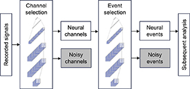
Figure 3. Spike detection method from Saif-ur-Rehman et al [100] and Okreghe et al [109]. The first CNN was employed to detect neural channels. Okreghe et al used multi-channel data as an input to their CNN while Saif-ur-Rehman et al applied their model to single-channel data. The next step involved applying a second CNN to the chosen neural channels in order to identify neural events and remove noise and artefacts. The identified neural events were then used for further analysis.
Download figure:
Standard image High-resolution image3.2. Detection of complex spikes (CSs)
Ideally, spike detection models can detect spikes at different scales and even under adverse conditions. However, Purkinje cells produce ‘CSs’ that show high misclassification rates with conventional algorithms due to their polymorphic complexity [93]. The role of CSs has been controversially discussed in the past. While it has been hypothesised that CSs play a significant role in motor timing [121] or performance-based motor learning [122], not all experiments in the past were conclusive in this regard [93]. Muller et al recently found that CSs modulate the simple spike output of Purkinje cells, which influences certain behaviour, such as eye saccades [123]. Since CSs could only be reliably detected manually by experts for many years, Markanday et al [93] developed a CNN for this purpose. Compared to usual spikes, CSs are rare events whose waveforms exhibit specific characteristics, as they are relatively long-lasting, polyphasic events, often showing inconsistency during a single recording. In [93], a human expert labelled the start and end points of CSs in 159 recorded Purkinje cells with 24 segments per cell, each with a length of 25 0 ms [93]. The famous U-Net [124] inspired the architecture of the utilised CNN. Given the reliability with which human experts reach a consensus on the presence of CSs, the input of the CNN was twofold: (i) band-pass filtered spikes with a frequency range of 300 Hz to 3 kHz; (ii) LFP with a frequency band of 30 Hz to 400 Hz [93]. With a kernel size of nine, they used by far the largest kernel of all CNNs described in this work, as CSs are longer events (∼10 ms) than usual spikes (∼1–2 ms) [93]. The method in [93] includes a three-step post-processing procedure to improve the system’s overall performance. The first step realigns the detected CSs. The second step maps spikes and LFP waveforms occurring within 2 ms after the CS start into a two-dimensional feature space using the uniform manifold approximation and projection algorithm [125]. Subsequently, DBSCAN was employed to identify spike candidates. Using this technique, usual spikes could be separated from CSs [93]. Combined with downstream post-processing, the model in [93] proved superior to a popular spike sorter and a PCA-based algorithm for CS detection, despite being trained with little data. Another method that was frequently applied in the past to detect CSs is the template matching-based alpha omega engineering multi spike detector (MSD) [126]. However, its performance was limited due to the inconsistent waveform characteristics of CSs [93]. According to Markanday et al, their method outperformed MSD [93].
4. Feature extraction
In 2017, Yang et al proposed an approach to extract neural features with PCANet [82], a DNN that utilises the basic principles from PCA. While PCA is a linear dimensionality reduction technique, a deep learning-based PCANet applies non-linearity across its layers. Features can be learned hierarchically and extracted locally in PCANet [82]. Moreover, PCANet runs faster than traditional PCA as it avoids the computationally demanding eigen-decomposition by applying filters directly to a given input. Yang et al considered these advantages to build a faster model that utilises PCA principles and overcomes the classical downsides of PCA [82]. Using conventional PCA, the extracted spikes and their corresponding eigenvalues were clustered by employing the k-means algorithm [82]. The cluster centres were then taken as spike templates and were shifted to create a Toeplitz matrix where the columns were used to train the PCANet [82]. In the subsequent stage, the resulting eigenvectors of PCANet were utilised as inputs for an SVM to classify spikes according to their underlying neuron. Following Yang et al [82], the proposed method had lower complexity than conventional methods, like PCA and k-means, but indicated no superior performance.
In 2020, Wouters et al [91] proposed a feature extraction method to resolve overlapping spikes in the feature space, a problem that often limits clustering methods in separating spikes from distinct neurons. In [91], an MLP was trained using the custom cost function in equation (1),

where g corresponds to the non-linear feature map, and si ⊕ sj denotes the superposition of spikes from two different neurons i and j. The hyperparameter κ was determined by a grid search and set to ten [91]. The first component of the cost function decreases by treating features as a linear operator on a linear combination, while the second term enhances the separation between spikes of distinct neurons in the feature space, thereby avoiding convergence to trivial solutions [91]. The MLP in [91] takes 300 features (30 samples × 10 spikes) as input and processes the data through two hidden layers with 600 and 60 units. The output layer has three units, and all layers use the ReLU activation function. The training set consisted of 50 000 waveforms, where three samples were created for each pair of neurons i and j: si, sj, and si ⊕ sj [91]. To create si and sj, random white noise was superimposed with artificial spikes, aligning them based on their highest peak and adjusting the time dimension to a specified window size of 30 samples. Creating si ⊕ sj involved randomly shifting the template of neuron i in relation to the spike template of neuron j [91]. Wouters et al could demonstrate that the trained MLP in [91] reliably resolves spike overlaps in the feature space, thereby improving subsequent clustering with k-means. This method and other models, which were dedicated to overlapping spikes, are revisited in section 7.3.
AEs are powerful tools for spike-denoising [127], data compression [128], and feature extraction, as we will see in this section. Basic architectures of AEs with varying depths can be seen in figure 4. The input signal is processed by the encoder module (layers with gradually decreasing size in figure 4) until it passes the coding layer (also called bottleneck; layers with three units in the middle of the AEs in figure 4) and is propagated through the decoder module that tries to reconstruct the input signal (bottom parts of the AEs in figure 4). As the encoder drastically reduces dimensions, the model creates a low-dimensional latent space that often facilitates clustering. In 2023, Ardelean et al [111] analysed different AE architectures, including shallow AEs, deep AEs, and LSTM AEs. The authors of [111] used synthetic data [2] (single-channel recordings with up to 20 active neurons) and experimental recordings [111] in their experiments. Among all architectures evaluated by Ardelean et al, the shallow AE performed best on the synthetic data, which can be attributed to the low data complexity (high SNR and no spike overlaps) [111]. This finding is consistent with standard deep learning principles, as the size (and layer complexity) of the hidden space should always be adjusted to the complexity of the problem [129]. Using the experimental data, this could be supported as the AE with eight hidden layers in the encoder and decoder achieved better results than the shallow AE [111]. Ardelean et al demonstrated that their model isolates 10 out of 17 distinct spike clusters in a specific synthetic recording [111]. However, other studies reveal that spike data with such ‘low complexity’ can be sorted precisely with other unsupervised machine learning-based methods, as Nadian et al [130] utilised t-SNE in combination with DBSCAN, achieving an accuracy of >90% on the synthetic data in [2] with up to 20 active neurons.
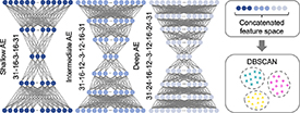
Figure 4. Ensemble method proposed by Eom et al [96]. (a) Shallow, intermediate and deep AE architectures. The numbers indicate the number of units per layer. (b) The bottleneck layers of each model consist of three units, and together they create a nine-dimensional feature space. Subsequently, this feature space is clustered using DBSCAN.
Download figure:
Standard image High-resolution imageIn 2020, Eom et al [96] presented a method to extract features with an ensemble of AEs based on the idea that models of different dimensions capture different spike characteristics. They detected spikes with amplitude thresholding [44], followed by obtaining the spikes’ gradient values, which is advantageous in signal processing tasks [131]. Subsequently, the spikes were temporally aligned to facilitate feature extraction. Eom et al found that shallow networks capture general spike attributes, while deeper networks better represent details of a given spike [96]. Hence, they applied the pre-processed signals to three differently sized AEs, which are shown in figure 4. The ReLU activation function was employed to add non-linearity to the hidden layers. The hidden codes of each model were concatenated to generate a nine-dimensional feature space, which was clustered using DBSCAN [96], as illustrated in figure 4. Eom et al achieved an accuracy of 99.81% on the widely-used synthetic data in [44] (overlapping spikes were excluded for this evaluation). Furthermore, multidimensional input (concatenated Tetrode-data) in a one-dimensional input vector improved the sorting accuracy from 96.58% to 98.27%, as the model could extract more valuable features [96]. Further considerations regarding the scalability of this and the following model can be found in section 7.1.
In 2021, Seong et al [103] also proposed an AE for feature extraction. Their method includes the following steps: detection, alignment, initial template generation, feature extraction, and clustering. To detect spikes, the dual vertex threshold method [132] was employed. Then, the initial spike templates were generated by using the first 100 aligned spikes in the data, and the number of centroids for clustering was determined [103]. The AE in [103] is detailed in table 6. The decoder network has a mirrored architecture to the encoder. Notably, L2-normalisation was applied to the last layer of the encoder as this facilitated clustering. Moreover, a ‘spike aware’ loss function was designed to assign more importance to the middle of spikes (peak and valley samples). For clustering, a k-means algorithm based on cosine similarity that is robust against false positives was utilised [103]. Using the synthetic data in [44], Seong et al reached an accuracy of 95.54%. It has to be considered that Seong et al evaluated their model using 5-bit weights and 7-bit activations, as the goal in [103] was to build an efficient hardware solution, which is described in section 7.2. As already observed in some detection models, performance in high-noise environments remains challenging [103], as a low SNR leads to stronger signal corruption, which increases the intra-class variance of spike features and thus complicates clustering.
Table 6. Model architecture of the encoder network in [103].
| # | Type | Dim. | σ(x) | Kernel | Stride |
|---|---|---|---|---|---|
| 0 | Input | 50 | — | — | — |
| 1 | 1D-Conv | 32 @ 25 | ReLU | 3 | 2 |
| 2 | 1D-Conv | 64 @ 13 | ReLU | 3 | 2 |
| 3 | 1D-Conv | 96 @ 7 | ReLU | 3 | 2 |
| 4 | Dense | 4 | — | — | — |
To address this problem, Radmanesh et al [107] built contractive AEs (CAEs), which include a contractive penalty term in the loss function, that penalises the Frobenius norm of the Jacobian matrix of the encoder activations, forcing the learned representations to exhibit invariance to minor variations in the input. The model architectures in [107] were optimised on each recording individually by using a grid-search algorithm. The smallest model applied to the data in [44] had a dense architecture with 72, 45, 20 and 3 units in each layer, while the biggest model, used for the data in [45] was equipped with 90, 70, 35 and 10 units, respectively [107]. Although this technique yields optimal results, it may also lead to models that are overly adapted. In contrast to [96] and [103], the authors of [107] utilised labels derived from a k-means algorithm to train an SVM for classification. Radmanesh et al outperformed several state-of-the-art methods, such as SPC [44], IronClust [63], and MountainSort4 [60] by achieving accuracies of 97% and 96% on two specific recordings from [44], 91% on the data in [108], and 87% on a recording from [45]—all while maintaining a faster processing speed [107]. Notably, the CAEs showed minimal sensitivity to the size of the training set, making them good candidates for even small datasets and online inference [107]. The benefit of using contractive loss could be further demonstrated, as simple AEs without contractiveness could not compete with the used CAEs [107].
5. Spike classification
This section presents straightforward classification models and more advanced solutions developed to address some of the mentioned challenges in spike sorting, such as overlapping spikes or limited prior information about the data. Supervised NNs require input (spike) and output (label) combinations to learn underlying data patterns but usually achieve higher accuracy than unsupervised models. Both methods can be combined, where unsupervised models are used during an initialisation phase to label a training set for the supervised model that can be trained subsequently to perform online spike sorting. This was also done for the spike detection models in [109] and [88], with Kilosort [21] as the utilised tool to generate binary pseudo-labels (‘spike’ or ‘no spike’). However, to sort spikes according to their underlying neuron, the spike IDs, e.g. ‘spike A’, ‘spike B’ and ‘spike C’, must be obtained. In 2019, Park et al [78] utilised an MLP for spike classification. The strategy in [78] is illustrated in figure 5. Park et al [78] used PCA and k-means to create pseudo-labels, using only the spikes in the data that were located closest to the centroids in the feature space to minimise labelling errors [78]. After training, the MLP assigns each spike with a label by using a Softmax layer with n units for n possible classes. The MLP in [78] has four hidden layers with 256 units each that use the hyperbolic tangent activation function,  . The results demonstrate that unsupervised pseudo-labelling with PCA and k-means combined with subsequent supervised classification yields better performance than only applying PCA and k-means or SPC [78]. However, the unsupervised training strategy limits the model’s classification performance. Accuracy increased from 51.55% to 99.55% on a specific recording when trained with the actual labels [78]. Thus, a change towards a more advanced unsupervised labelling strategy may result in fewer erroneous labels and therefore could improve performance. The scalability of this and some of the following approaches are discussed in section 7.1.
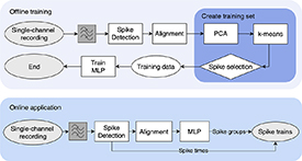
Figure 5. Spike sorting strategy proposed by Park et al [78]. Offline training: after band-pass filtering of the signal, spikes get detected and aligned. PCA and k-means are used for feature extraction and clustering. Subsequently the MLP is trained with the spikes that are closest to the centroids in the feature space to minimise labelling errors. Online mode: after being trained, the MLP can classify detected and aligned spikes.
Download figure:
Standard image High-resolution imageIn 2020, Li et al [98] also worked on the classification of spike waveforms. For the synthetic data [44], Li et al used the true labels available with the dataset to train their model, varying the size of the training set between 5% and 50%. However, they did not mention spike alignment, even though this step is of big importance as the spikes have cluster-specific shifts with respect to the given ground-truth information. If these shifts are not corrected by an alignment procedure, there is a risk that the respective deep learning model learns these characteristic peak positions, which are not present in real scenarios. Hence, the model in [98] could be biased in this regard. The architecture of the CNN in [98] is summarised in table 7. Li et al regularised their model using batch normalisation and dropout. Evaluated on the data in [44], the CNN [98] achieved high accuracy, performing slightly better than the MLP in [78] (even when trained with the true labels), at the expense of higher computation. However, depending on whether the spikes were aligned before model training or not, the possible bias mentioned above may have led to falsely promising results. Naturally, more training data increased performance. Nevertheless, even with 170 labelled spikes (5% of the available data), the CNN achieved >99% accuracy for most synthetic signals [98]. Using real extracellular data [98], the average accuracy of this CNN dropped to 96.53%, which may be due to inherent challenges of real data, such as class imbalance and more realistic noise. Moreover, some recordings in [98] do not contain enough data from a single neuron to train the model [98]. Using the experimental data, the CNN in [74] was trained with spikes that were pre-sorted using SPC and manual re-sorting [44]. Therefore, the proposed method resembles the one in [78], as an unsupervised method was used to create pseudo-labels. Note that for the data in [98], spikes were aligned before pre-sorting with SPC.
Table 7. Architecture of the CNN in [98].
| # | Type | Dim. | σ(x) | Kernel | Stride |
|---|---|---|---|---|---|
| 0 | Input | 64 | — | — | — |
| 1 | 1D-Conv | 32 @ 64 | ReLU | 3 | 1 |
| 2 | 1D-Conv | 64 @ 64 | ReLU | 3 | 1 |
| 3 | Pooling | 64 @ 32 | — | 2 | 2 |
| 4 | 1D-Conv | 128 @ 32 | ReLU | 3 | 1 |
| 5 | Pooling | 128 @ 16 | — | 2 | 2 |
| 6 | 1D-Conv | 128 @ 16 | ReLU | 3 | 1 |
| 7 | Dense | 300 | ReLU | — | — |
| 8 | Dense | 100 | ReLU | — | — |
| 9 | Dense | n | Softmax | — | — |
In 2023, Wang et al [113] proposed a convolutional LSTM for spike classification. The detection unit, consisting of two CNNs, was explained in section 3. The output of the second CNN defines the start and end points of a potential spike with a length of 40 samples. The authors of [113] split each predicted waveform (40 × 1) into seven sliding windows (10 × 7) with an overlap of five samples for each window. This was then applied to an LSTM layer that created seven time-series features. These features were spliced into a 2D-feature matrix (7 × 7) to construct the input for the subsequent convolutional layers [113]. The architecture of the model in [113] is shown in table 8. Comparing the results from Li et al [98] and Wang et al [113] on the synthetic data [44] reveals that both models performed similarly. Li et al [98] reached 99.08% accuracy using 5% of the data for training, while Wang et al [113] achieved 98.85%; using 40% of the data for training, they reached an accuracy of 99.58% and 99.55%, respectively. By processing ten individual channels of the experimental data in [99] containing the activity of three, four and five neurons, Wang et al reached an average accuracy of 94.77% with 50% of the available data used for training, whereas the CNN from Li et al [98] reached 95.66% on the same channels.
Table 8. Model architecture of the LSTM-CNN in [113].
| # | Type | Dim. | σ(x) | Kernel | Stride |
|---|---|---|---|---|---|
| 0 | Input | 10 × 7 | — | — | — |
| 1 | LSTM | 7 | — | — | — |
| 2 | 2D-Conv | 25 @ 7 × 7 | ReLU | 3 × 3 | 1 × 1 |
| 3 | 2D-Conv | 50 @ 7 × 7 | ReLU | 1 × 1 | 1 × 1 |
| 4 | Dense | 50 | — | — | — |
| 5 | Dense | 25 | — | — | — |
| 6 | Dense | n | Softmax | — | — |
5.1. Classification of overlapping spikes
Recent studies, like the one by Liu et al [106] in 2022, or the one by Zhang et al [115] in 2023, focused explicitly on the problem of overlapping spikes. Both of these studies also did not mention spike alignment, which may introduce the same bias as mentioned above. The model used in [106] offers a combination of CNN and LSTM, which is detailed in table 9. Batch normalisation was utilised for the convolutional layers to regularise the model. Notably, a Softmax layer with m units was utilised to classify the input: one class for each spike group and additional units for all possible overlapping combinations of spikes from two neurons. The model in [106] could distinguish between these classes as it was trained with augmented data consisting of single spikes and artificial overlaps. Compared with the study in [98], results could be improved, especially on spike collisions [106]. The proposed technique to address overlapping spikes is discussed in section 7.3.
Table 9. Model architecture of the LSTM-CNN in [106].
| # | Type | Dim. | σ(x) | Kernel | Stride |
|---|---|---|---|---|---|
| 0 | Input | 64 | — | — | — |
| 1 | 1D-Conv | 32 @ 64 | ReLU | 3 | 1 |
| 2 | 1D-Conv | 32 @ 64 | ReLU | 3 | 1 |
| 3 | Pooling | 32 @ 32 | — | 2 | 2 |
| 4 | LSTM | n/s | — | — | — |
| 5 | Dense | 300 | ReLU | — | — |
| 6 | Dense | 100 | ReLU | — | — |
| 7 | Dense | m | Softmax | — | — |
Zhang et al [115] addressed the spike classification problem using the Log-Mel spectrogram and a CNN. Spectrograms are widely used in signal processing, particularly for speech recognition and music analysis. Furthermore, logarithmic scaling in the spectrogram enhances its informativeness and adaptability for various signal-processing applications. The procedure in Zhang et al [115] has two parts. The first part utilises the short-time Fourier transformation to acquire the signal’s spectrogram, which was converted into a Log-Mel spectrogram to reduce the amount of data while extracting advantageous features [115]. In the second part, a CNN is utilised to process the spectrogram. This CNN contains four convolutional layers with 2 × 64 and 2 × 128 filters, two average pooling layers, and two dense layers. As in [106], a Softmax layer predicts one of m classes [115]. This was also achieved by training the model on both single-spike waveforms and artificial overlaps. The size of the training set is not specified in this work. Using the data in [44], Zhang et al reached an accuracy of 95.74% [115], whereas Liu et al [106] reached more than 99.5%, suggesting that the use of spectrograms may not provide additional benefits for deep learning-based spike sorting. A similar finding comes from Ardelean et al, who also demonstrated that spectral analysis does not offer an advantage in capturing distinct spike features [111].
5.2. Spatiotemporal classification models
Rácz et al [88] proposed CNNs using 2D- and 3D-input to sort spikes obtained with a 128-channel HD-MEA. Figure 6(a) illustrates how spikes of different neurons may appear spatially on a 32 × 4 electrode grid at their negative amplitude peak. Figure 6(b) shows how a spike evolves in a spatiotemporal way and how these patterns can be used for signal analysis. The model in [88] that utilises 2D input only took spatial data as input, with spikes at their amplitude peak (cf figure 6(a)). More precisely, frames with an offset of 1–2 samples were used, as these frames yielded the best results [88]. A model with 3D input was also created, using six frames per spike, where each adjacent frame was five samples apart to keep the training time low [88]. The architecture of the CNN in [88], using 3D input and assuming there are n actively firing neurons in the recording, is displayed in table 10. For the data used [89], n ranged from 23 to 46, determined with Kilosort [21], which was also utilised to generate pseudo-labels for the supervised models. The results indicate that the 3D-model provides higher accuracy than the 2D-model, as unique temporal spike characteristics provide crucial information [88]. As for the synthetic data mentioned above, pre-sorting with Kilosort also resulted in cluster-specific shifts, that should have been corrected by alignment before network training. However, this was not taken into account in this study either, which also potentially skewed the results. Nevertheless, the method of Rácz et al shows significant advantages over the aforementioned classification models, as the CNN in [88] processes many channels at a time by using a compact network architecture. Another issue was identified in this study: even though classes are imbalanced, the examples per class were not rebalanced for training, which can lead to a deep learning model that weights frequently occurring classes more heavily than examples of rare classes. This was also neglected by the studies mentioned above that were using experimental data [98, 106, 113]. Rácz et al also investigated the feasibility of spike predictions before they appear in the signal. This would be useful for BCIs as the delay between sorting and actuation could be reduced. It was shown that the initial waveform (not containing the peak voltage) enabled spike classification to a certain extent, indicating that the initial spike frames contain essential information of a unit’s identity. However, predictions before the firing of a neuron were not possible [88]. More reflections on the scalability of this and the following model can be found in section 7.1.
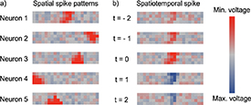
Figure 6. Simulated HD-MEA recording. (a) Five distinct neurons in an extracellular recording at their negative amplitude peak, captured with an HD-MEA (32 × 4 electrodes). Each neuron produces a characteristic voltage pattern. (b) Spatiotemporal spike data of Neuron 1 over five consecutive time-steps. Peak negative amplitude at t = 0.
Download figure:
Standard image High-resolution imageTable 10. Model architecture of the CNN in [88].
| # | Type | Dim. | σ(x) | Kernel | Stride |
|---|---|---|---|---|---|
| 0 | Input | 32 × 4 × 6 | — | — | — |
| 1 | 2D-Conv | n @ 32 × 4 | Linear | 4 × 2 × 6 | 1 × 1 × 1 |
| 2 | Dense | n | Linear | — | — |
| 3 | Dense | n | Softmax | — | — |
In 2022, Yi et al [105] also proposed a multi-channel spike sorting model. The data were captured using 64 channels, 49 of which were processed in [105]. The utilised recording shows the activity of 27 neurons. MountainSort [59] was used for labelling, which produced data batches of 49 × 180 samples for all relevant events (180 samples = 6 ms). Yi et al [105] reduced the size of spike snippets to 49 channels x 30 timesteps, as this duration was sufficient to capture relevant spike features [105]. Naturally, a smaller input leads to faster processing of the DNN. However, instead of using every fifth sample from each spike waveform, as Rácz et al did in [88], Yi et al processed the entire waveform to avoid losing important spike features. The input waveform was divided into five sub-snippets, leading to an input size of 49 × 6 × 5 per spike. According to Yi et al, this approach prevents the model from overfitting to certain noises and guides it to better focus on learning spatial features [105]. The CNN used in [105] is detailed in table 11. The authors in [105] could attain a testing accuracy of 93.1% employing full-precision weights and 86.1% using quantised weights with 4-bit precision [105]. The hardware implementation of this approach is briefly discussed in section 7.2.
Table 11. Model architecture of the CNN in [105].
| # | Type | Dim. | σ(x) | Kernel | Stride |
|---|---|---|---|---|---|
| 0 | Input | 49 × 6 × 5 | — | — | — |
| 1 | 2D-Conv | 2 @ 46 × 2 | ReLU | 4 × 4 × 5 | 1 × 2 × 1 |
| 2 | 1D-Conv | 2 @ 45 | ReLU | 4 | 2 |
| 3 | Dense | 27 | Softmax | — | — |
5.3. Spike classification with GANs
In a GAN, adversarial representation learning can be utilised by employing a generator to produce realistic data samples and a discriminator to distinguish between genuine and generated samples. This approach helps in acquiring meaningful data representations and can improve spike sorting quality by extracting robust features from limited labelled data. In 2019, Wu et al [84] developed a semi-supervised spike classification method called few-shot spike sorting (FSSS). They presented a semi-automatic threshold-based labelling technique called DidacticSort to create cluster candidates for the spikes in the utilised data. Experiments were obtained with 50, 100 and 200 labelled spikes from the synthetic data in [44]. The encoder (generator network) of FSSS is detailed in table 12. Two residual blocks, which can be seen as skip connections that add the input directly to the output, were employed to avoid vanishing gradients. The encoder has two outputs: (i) an encoded vector y to predict one of n cluster labels; (ii) a hidden code z (low-level feature representation). As the output of the encoder q is twofold, Wu et al [84] used two discriminator networks called  and
 , which are two-layer MLPs with 512 units. The GAN was trained following a three-step algorithm, which is illustrated in figure 7. The authors of [84] successfully categorised spikes within the utilised synthetic data: using 50 labelled spikes from a recording with noise a standard deviation of 5%, an accuracy of 97.7% was reached; by increasing the number of labelled spikes to 200, the accuracy improved to 98.2%. In the presence of noise with a standard deviation of 20%, they reached accuracy levels of 66.4% (50 labelled spikes) and 85.5% (200 labelled spikes) [84]. Also tested on experimental data, it was demonstrated that training the GAN on a particular waveform with only a ‘few shots’ was sufficient to recognise similar spikes in inference mode. In the following, it is discussed that a GAN approach can also be carried out in a fully unsupervised way.
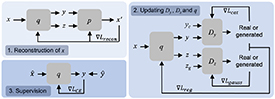
Figure 7. Training procedure of the model in [84]. (1) The encoder q and the decoder p are trained to reconstruct given spikes by minimising the reconstruction loss Lrecon, where x and x′ are the unlabelled spikes and their reconstructed versions, respectively. (2) The discriminators  and
 are trained to distinguish the generated y and z from samplings of the categorical distribution yc and d-dimensional Gaussian distribution zg by adjusting the model weights according to Lcat and Lgauss. Furthermore, q is trained to better fool
 and
 by minimising the regularisation loss Lreg. (3) The supervised part comes last, when q is updated by minimising the cross-entropy loss LCE on a mini-batch of labelled spikes
 , where the labels
 were obtained by DidacticSort.
Download figure:
Standard image High-resolution imageTable 12. Model architecture of the encoder in [84].
| # | Type | Dim. | Kernel | Stride |
|---|---|---|---|---|
| 0 | Input | 64 | — | — |
| 1 | 1D-Conv | 64 @ 64 | 1 | 1 |
| 2 | Residual block | 256 @ 64 | 3 | 1 |
| 3 | Residual block | 256 @ 64 | 3 | 1 |
| 4 | Dense | 512 | — | — |
| 5 | Dense | 512 | — | — |
| 6.1 | Dense (y) | n | — | — |
| 6.2 | Dense (z) | d | — | — |
In 2020, Ciecierski [94] proposed a similar method for spike sorting that also relies on the interplay between a generator network and two discriminators. Similar to [84], pre-processing in [94] involved spike detection and alignment to facilitate sorting with the used model. The encoder in [94] processes the input through two dense layers with 100 units each, before the model splits into a categorical output and a Gaussian output. Ten units were used for the categorical output, as it was assumed that no more than ten distinct neurons were firing in the respective recording. Notably, this number represents an upper limit and does not determine the number of active neurons in the recording [94]. Three units were chosen for the Gaussian output. For the first two hidden layers, the author in [94] applied the exponential linear unit activation function,  if
 , else
 , with
 as a hyperparameter. The decoder was designed the same way as the encoder but with an additional hidden layer after both inputs. Furthermore, Ciecierski used a ‘spike aware’ loss function, similar to [103]. The ability to enforce both desired distributions (categorical and Gaussian) in the latent space was achieved by using discriminator networks during training, similar to the work of Wu et al [84]. Both the categorical and the Gaussian discriminators were designed as 3-layer MLPs with 100 units in the hidden layers [94]. The training setup for the proposed GAN is similar to the work in [84], but has no supervised part. The model in [94] could identify nine distinct spike waveforms during training, validation and testing, using experimentally obtained recordings [95]. Unfortunately, this model was not evaluated on the widely-used synthetic data in [44], and thus the performance of FSSS [84] cannot be compared with Ciecierski’s model.
6. Integrated systems
Recently, Meyer et al [116] and Zacharelos et al [117] proposed lightweight MLPs for simultaneous spike detection and spike classification using single-channel recordings and supervised learning. Also, Rokai et al [101, 112] presented a mixture of supervised and unsupervised, computationally more intensive solutions, for integrated multi-channel spike sorting by employing more complex network configurations.
6.1. Integrated systems for single-channel recordings
In 2023, Meyer et al [116] proposed DualSort, which was trained using synthetic and real extracellular recordings, labelled with the spikes’ IDs and timings. Data augmentation with noise was employed to create an extensive training set, similar to the work in [118]. Furthermore, the spikes were extended by shifting them along the time axis in order to train the model to become shift invariant. This enabled classifying spikes at multiple adjacent time steps [116]. The architecture of this model is detailed in table 13. The first output layer was used for spike detection and localisation at twenty different positions in the input, indicating the exact spike timing, while the second output layer predicts one of n spike classes [116]. Both output layers contain an additional unit to indicate when no spike is present [116]. Dropout, batch normalisation and early stopping were utilised to regularise the model. Meyer et al also designed a post-processing algorithm that verifies the output of the MLP by validating whether the refractory period of individual neurons was violated, and by calculating the mode of the last 20 predictions to only keep the most frequent classification [116]. DualSort offers high accuracy (98.04% with post-processing; 97.34% as a single-shot model) on the widely-used synthetic dataset [44] outperforming other advanced spike sorting models like WMsorting [133]. The spike times could be predicted precisely as well (84.07% of all predictions were exact; wrong predictions had a mean deviation of 1.1 samples @ 24 kHz). Misses in this regard were mainly caused by overlapping spikes. Using the experimental recordings in [98], it was even possible to outperform the CNN from Li et al [98], especially when trained with little data. The post-processing algorithm helped to increase the robustness against misclassifications, as these often stood out as outliers in larger prediction sequences [116]. The scalability of this and other integrated systems is discussed in section 7.1.
Table 13. Model architecture of the MLP in [116].
| # | Type | Units | σ(x) |
|---|---|---|---|
| 0 | Input | 25 | — |
| 1 | Dense | 100 | ReLU |
| 2 | Dense | 100 | ReLU |
| 3.1 | Dense | 21 | Softmax |
| 3.2 | Dense | n + 1 | Softmax |
Later in 2023, Zacharelos et al [117] also presented an MLP for integrated spike detection and classification, which has many similarities with DualSort [116]. However, the authors of [117] also proposed a hardware implementation, which is briefly described in section 7.2. Neurocube [108] was utilised in [117] to generate synthetic extracellular recordings with three active neurons. Different MLP architectures were investigated in [117], where the optimal solution had two hidden layers with 24 and 16 units. The output layer of the model in [117] resembles the second output layer of DualSort [116], as three units were used to indicate activity from the three firing neurons and one unit was utilised to indicate pure noise activity. Both hidden layers apply the ReLU activation function, and the Hardmax activation function was applied to the output layer [117]. Hardmax, also known as the argmax function, identifies the unit with the highest value, which saves resources compared to Softmax. For regularisation, the authors in [117] used early stopping and L2-regularisation. Tested on the synthesised recordings, Zacharelos et al reached an accuracy of 96%. The model in [117] has a leaner architecture than DualSort but was optimised and tested on a single dataset, which does not allow any conclusions on the generalisation of the model in [117]. Additionally, the model in [117] cannot gain exact information regarding the spike timing. Hence, if the spike trains need to be reconstructed by the network outputs, DualSort has a slight advantage in spike time accuracy.
6.2. Integrated systems for multi-channel recordings
In 2021, Rokai et al [101] presented ELVISort, an integrated multi-channel spike sorting system based on a variational AE (VAE). In VAEs, loss is augmented to force the hidden code to have a normal distribution, which regularises the model and leads to more consistent latent representations. The encoder contains two branches of Bi-LSTM and 2D-convolutional layers with dense layers at the end [101]. A Bi-LSTM operates by processing inputs in forward and backward directions through the hidden layers before the outputs get combined at each time step. The dense layers in ELVISort are followed by three branches. The first branch reconstructs the input and consists of LSTM and attention layers, as this improved the generalisibility of ELVISort [101]. Attention layers allow to selectively focus on specific segments of the input data dynamically, rather than treating all inputs the same way. The second branch is for classification, which is used to fine-tune the model for spike detection using a Softmax layer with two units (‘spike’ or ‘no spike’), while it was tuned to the number of clusters n in the respective recording for sorting (this is the only supervised part of the network). The third branch is for clustering, where Student’s t-distribution was utilised to assign soft labels during training and k-means for centroid initialisation. During training, the reconstruction capability of ELVISort was given the highest priority. ELVISort [101] was evaluated on three experimental datasets using the  -Score, a statistical measure used to evaluate the performance of a classification model that calculates the harmonic mean of precision and recall and ranges from zero (minimum) to one (maximum). Using the data in [102], ELVISort achieved an
 -Score of 0.964, which is competitive to several state-of-the-art models, such as Kilosort (F1: 0.98) and IronClust (
 : 0.97) [101]. Using the hybrid dataset in [46], ELVISort reached an
 -Score of 0.81, a comparable result to SpyKING CIRCUS, Kilosort2, and IronClust, all achieving an
 -Score of 0.83 [101]. Although the unsupervised part of ELVISort exhibited a commendable capacity for detection and sorting, the cluster-specific accuracies were loosely correlating with the average SNR of the cluster, suggesting that the performance bottleneck could be in the feature extraction part of the algorithm [101].
In 2023, Rokai et al presented a new solution for integrated spike sorting [112], using tensor processing units (TPUs) to accelerate sorting. They developed a semi-automatic procedure where spikes were averaged from a specific cluster to identify the primary channel number, which was verified by a human expert [112]. The model consists of a self-supervised and a supervised model. The self-supervised model takes 105 features as input and processes the data through three residual blocks, four 1D-convolutional layers and one dense layer at the end, where it outputs 32 features (spike embedding). Batch normalisation was used for regularisation, and the model utilised the leaky ReLU activation function,  if
 , else
 , with
 as a hyperparameter that controls the slope for negative inputs. Nearest-neighbour contrastive learning NNCLR [134] was chosen as the self-supervised method in [112]. The training procedure of the self-supervised method is illustrated and explained in figure 8(a). The model in [112] was trained with multiple recordings at once to increase generalisability. Furthermore, spikes were augmented using scaling and jittering to extend the training set with similar input pairs. Each mean waveform’s embedding is then used as a label for the supervised model, displayed in figure 8(b). MobileNetV2 [135] was the chosen architecture for the supervised model, as it supports edgeTPU hardware, and is well suited for applications with limited resources. The key concepts in MobileNetV2 are depth-wise separable convolutions, inverted residuals, and linear bottlenecks. The initial convolutional layer is followed by a series of bottleneck layers where the number of channels is expanded, depth-wise convolutions are carried out, and the dimensions are reduced again. The last convolutional layer is pooled, followed by a Softmax layer for classification. A single-shot detector (SSD) approach called SSDLite [135] was used to recognise spikes in the signal. SSD utilises predefined anchor boxes to predict class probabilities and box offsets at various feature map locations, refining these predictions during training with localisation and classification losses and applying non-maximum suppression (NMS) to remove overlapping boxes. SSD represents an effective alternative to the spike localisation method presented in [113], where two CNNs were utilised to detect and localise spikes in the signal, or DualSort [116], where spikes were detected, localised and classified according to their underlying neuron. However, in contrast to [116], the model in [112] does not classify spikes directly but creates a reduced feature space that is clustered subsequently. This method has the advantage of increased generalisability because the model is not restricted to certain cluster assignments or specific electrode geometry [112]. PCA was applied to reduce the feature dimensions from 32 to 10 to enhance future data adaptability and mitigate overfitting [112]. For clustering, Rokai et al carried out experiments with Isosplit5 [136], a time-efficient algorithm that does not require hyperparameters, and agglomerative clustering, which is a hierarchical method. It was demonstrated in [112] that the proposed algorithm can be used for spike detection, achieving an average accuracy of 93% on the data in [43, 62], performing better than other state-of-the-art techniques like Kilosort (77%), MountainSort4 (88%) or SpyKING CIRCUS (88%). Using two recordings of [46], the sorting accuracy of the model in [112] was 86% and 42%, whereas SpyKING CIRCUS reached 91% and 54%, respectively. As the self-supervised model processes pre-selected spike waveforms, it can be seen as input-source agnostic, which is a massive advantage in terms of flexibility [112]. One limitation of this model is the processing of overlapping spikes, as the NMS post-processing was not optimised for separating such events [112].
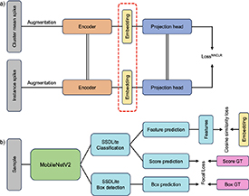


Figure 8. Training scheme of the model from Rokai et al [112]. (a) The encoder of the self-supervised model takes an instance spike and a cluster mean spike as input and creates two different feature embeddings. These embeddings are then processed by a projection head. By applying NNCLR, the contrastive loss is calculated to pull embeddings from positive input pairs closer together or push them further apart for negative input pairs. Once trained, the model creates similar embeddings for similar spikes. (b) The supervised model is based on MobileNetV2 and splits into a classification and detection branch using SSDLite. Following the classification branch, the model predicts the feature embeddings of single samples. Based on the cosine similarity loss between the predicted features and the embeddings provided by the self-supervised model, the weights of the model get adjusted. Furthermore, SSDLite predicts the score and box, compares it with ground truth (GT) by using focal loss, and adjusts the parameters accordingly. The box refers to the localisation of a spike within the sample, whereas the score prediction indicates whether a spike is present in the box or not.
Download figure:
Standard image High-resolution image

7. Discussion
Deep learning models have been utilised to solve specific problems in the spike sorting pipeline, which were explored in sections 3–5. Moreover, integrated systems were covered in section 6. MLPs are the simplest type of DNNs used in integrated spike sorting [116, 117]. They require few resources but have been optimised for single-channel data so far. The authors of [88, 101, 105], among others, demonstrated the advantages of convolutional layers in spike sorting. While 1D-convolutional layers were utilised to find temporal patterns in single-channel data [98, 103], 2D- convolutional layers could be used to process HD-MEA data spatiotemporally [88, 101, 105]. LSTMs have not yet been promising in detecting spikes, but could improve the temporal spike pattern recognition in some classification models [106, 113]. AEs, on the other hand, have demonstrated their effectiveness for unsupervised feature extraction [96, 103, 107], where they have been applied to reduce data dimensions to facilitate clustering. Notably, certain layer types, such as convolutional or LSTM layers, have been integrated into AEs to enhance performance [101, 103]. Furthermore, GANs have been proposed for spike classification with a semi-supervised [84] and a fully unsupervised solution [94]. GANs utilise adversarial representation learning, effectively categorising spikes with minimal or no labelled data by disentangling label information from extracted features. This approach further reduces the need for manual intervention and is especially useful on data with limited prior information. Generally, model architectures have been optimised with regard to specific recordings. This was often done analytically, by using grid search algorithms [107], but also heuristically [78]. It must be noted that the ability of the model to generalise to new data always depends on the quality and complexity of the data on which it has been optimised, even if it has been trained on the new data.
Table 14 provides the reader with a concise descriptive table that summarises the advantages, limitations and real-world applicability of certain deep learning models discussed in this work. Table 1 lists all datasets used in the respective studies, giving an overview of which algorithms may be suitable for comparative analyses. However, comparisons between models tested on the same dataset should be made cautiously, considering that many research groups tested their models on certain parts of the datasets. Moreover, algorithms were trained using different approaches: (i) supervised; (ii) semi-supervised; (iii) unsupervised, with differently sized training sets. Depending on the technique used, this significantly impacts the results. In this survey, the results are not compared in tabular form to avoid erroneous conclusions. Instead, it discusses how the presented solutions overcome several challenges and requirements mentioned in section 1.3, points on possible future directions and presents the first hardware implementations of deep learning-based spike sorting models.
Table 14. Key attributes of certain spike sorting algorithms: advantages, constraints and practical applications.
| References | Approach | Advantage | Drawback | Application |
|---|---|---|---|---|
| [100] | Two CNNs for channel selection and spike detection | Generalized solution to the spike sorting problem | Limited to single channel recordings | Universal channel tracking across species, brain regions and electrodes |
| [93] | CNN for CS detection | Accurately detects complex spikes with limited training data | Relies on several post-processing steps | Could improve neural decoding in BCIs |
| [96] | AE-Ensemble for feature extraction | Improved feature extraction through the use of multiple AEs | Not evaluated on overlapping spikes | Enhances spike sorting accuracy, especially with multi-dimensional inputs |
| [103] | Convolutional AE for feature extraction | Efficient model using low-bit weights and activations | Performance degrades in high-noise environments due to low SNR | Suitable for spike sorting in resource-constrained hardware systems |
| [78] | MLP for classification | Unsupervised pseudo-labelling enabled fully automatic supervised sorting | The labelling technique (PCA + k-means) limits the sorting accuracy of the MLP | Real-time spike classification |
| [105] | CNN for classification | Spatiotemporal sorting | Only validated on one HD-MEA dataset | On-chip sorting, enabled through a low-parameter model |
| [116] | MLP for integrated spike sorting | Bypasses several steps in the spike sorting pipeline | Sensitive to overlapping spikes | Real-time spike detection and sorting using a lean model architecture |
| [101] | VAE for integrated spike sorting | Various layer types such as convolutional and Bi-LSTM layers improve accuracy | Computationally heavy | Integrated spike detection and classification using HD-MEA data |
7.1. Scalability
For spike detection, models have been trained with millions of labelled waveforms and could be used universally. The authors of [85] presented a CNN for neural channel selection that can be applied to different subjects, species, brain areas and electrode types. This is beneficial for BCI applications in order to track useful channels. By using a second CNN [100], it was possible to remove background activity from the recorded channels which drastically reduced the number of waveforms for subsequent analysis. To gain insight into the computational complexity of the models in [85] and [100], the authors of this work reconstructed them using Python and TensorFlow and derived the total number of model parameters and the required floating-point operations (FLOPs). Spikedeeptector [84] and BAR [100] use 110 735 and 42 302 parameters and require 4157 178 and 1069 612 FLOPs, respectively. Ideally, CSs should also be detectable with BCIs, especially with implanted electrodes at the cerebellum, where CSs occur frequently. Hence, integrating CS detection into scalable multi-channel detection models, or integrated systems, is desirable for real-world applications in the future.
Certain feature extraction and classification models were also reconstructed within this survey to investigate their resource consumption. The results are displayed in table 15. Thirty-two units were assumed for the LSTM layer in [106], as this was not specified in the respective paper. Notably, all models in table 15 reached an accuracy above 95% on the utilised data. It is apparent that the ensemble learning model from Eom et al [96] requires the fewest parameters and the lowest number of FLOPs, even though Eom et al used three dense AEs. At this point, it should be noted that only the encoder modules of the AEs were reconstructed for this estimation, as the decoders are not required during inference. The resource consumption of the model in [96] is higher overall, considering the whole spike sorting pipeline, as the AE ensemble is employed only for feature extraction and additional modules for spike detection, temporal alignment, gradient determination and clustering are required. Table 15 reveals that the classification models in [78, 98, 106, 113] require significantly more parameters and FLOPs due to more complex network configurations. Notably, the size of the input vector plays a decisive role in this regard. Using the data in [44], the CNN in [98] classifies aligned spikes with a size of 64 samples, resulting in the resource consumption displayed in table 15. However, reducing the input spikes to the more ‘important’ samples (peak and valley), like in [116], where only twenty-five samples were used, the required memory and computation of the model in [98] shrink to 227 631 parameters (−63%) and 1552 698 FLOPs (−73%), respectively. Nevertheless, the total resource consumptions of the above models increases by the computational effort required for spike detection and alignment. This is not the case for the model in [116], as this is an integrated system. However, since the same spike is processed several times by the same network in [116], ultimately there are more FLOPs per spike than those presented in table 15. In practice, this results in a trade-off between model robustness, gained through the described post-processing, which also takes a small amount of computation, and resource efficiency, calibrated based on the model step size.
Table 15. Deep learning models trained on single channels of the synthetic data in [44] and their resource consumption.
| References | Authors | Parameters | FLOPs |
|---|---|---|---|
| [78] | Park et al | 206 595 | 412 163 |
| [96] | Eom et al | 2729 | 5353 |
| [98] | Li et al | 611 631 | 5788 250 |
| [106] | Liu et al | 52 414 | 501 060 |
| [103] | Seong et al | 27 556 | 430 276 |
| [113] | Wang et al | 125 957 | 395 968 |
| [116] | Meyer et al | 16 025 | 31 950 |
Scaling the discussed single-channel models up to HD-MEA recordings may significantly increase computation, and is an important subject of future research. Other classification models have already proven scalable using HD-MEA data by utilising spatiotemporal features for spike sorting. To better understand the efficiency of multi-channel models, the models from Rácz et al [88], Yi et al [105] and Rokai et al [101], were also reconstructed to estimate the required resources. The results are displayed in table 16. For both classification networks [88, 105] in table 16, it was assumed that there are twenty-seven active neurons in the recording. Table 16 demonstrates the effect of both a small number of filters and dimensionality reduction, as Yi et al [105] used only two filters and two convolutional layers, effectively shrinking dimensions. In contrast, Rácz et al [88] utilised one convolution, matched the number of filters with clusters in the data, and kept dimensions, resulting in a larger model. However, this does not imply that the model in [105] is fundamentally preferable, as the models were not tested on the same data. It may well be that the narrow architecture of the model in [105] would fail when processing the data used in [88]. Nevertheless, table 16 shows that spatiotemporal data processing can take less memory and processing power than channel-wise analyses (cf table 15).
Table 16. Deep learning models trained on HD-MEA data and their resource consumption.
| References | Authors | Channels | Parameters | FLOPs |
|---|---|---|---|---|
| [88] | Rácz et al | 128 | 561 978 | 3132 783 |
| [105] | Yi et al | 49 | 6876 | 36 176 |
| [101] | Rokai et al | 128 | 5315 139 | 275 713 102 |
Heavy models require external processing to ensure online sorting. Therefore, collected data must be transmitted to an external processor. In general, all described DNNs in this work can be run utilising a conventional CPU/GPU setup. Notably, the single-channel models presented in table 15 can also process multi-channel data using modern deep learning frameworks and optimised hardware that supports parallel processing, e.g. with GPUs. CNNs benefit most from parallel processing as filters can be applied across the entire input at the same time. MLPs benefit moderately from parallel computing, while RNNs are restricted in this regard as they depend on sequential processing. Irrespective of the model type, the following must be considered: if parallel processing is applied to a supervised single-channel classification model in order to process several channels simultaneously, the model must be trained on all spikes in all channels, and the model architecture must be adjusted accordingly. ELVISort [101], is a sophisticated integrated system that requires drastically more FLOPs and parameters than the single-channel models described above. Running ELVISort on a Windows PC using an i9-7920X with 64GB RAM and NVIDIA GeForce RTX 2080 Ti GPU, it was possible to sort spikes from 64 channels 15.71 times faster than the sampling rate [101]. Using the same setup, other state-of-the-art solutions were not that efficient: IronClust was 7.11 times faster than the sampling rate, Kilosort2 was 6.94 times faster, MountainSort4 was 2 times faster, and SpyKING CIRCUS was even slower than the sampling rate [101]. This shows that even heavy deep learning models can run faster than leading state-of-the-art solutions in spike sorting. To accelerate the performance of the model presented in [112], an edgeTPU chip was used that requires a comparatively small amount of energy (1 Watt/2 Tera Operations per second). An edgeTPU is a specialised application-specific integrated circuit (ASIC) that uses a TPU. As the post-processing (NMS and clustering) is not supported by TPU, processing can be divided into two parts: (i) spike detection and feature extraction with TPU; (ii) NMS and sorting on CPU. As the first part requires a quantised model, the model parameters were quantised from 32-bit floating values to 8-bit integers. A quantisation-aware training method was used to minimise the performance drop during this process [112]. Data-wise, the system presented in [112] can be trained on multiple recordings simultaneously, which highly improves generalisation. To summarise, the presented setup [112] is a step towards the integration of DNN-based spike sorting for BCIs.
7.2. Hardware implementations
On-chip processing can be done using field programmable gate arrays (FPGAs) [103, 132, 137, 138] and ASICs [139–142]. Several constraints must be considered regarding implantable brain chips: the power utilisation should not exceed 10 mW, the implant size should not be higher than 1 cm2, and energy dissipation should not raise the temperature of the surrounding cells by more than 1 °C [143, 144]. The BNN for single-channel classification by Valencia and Mohammad [42] was implemented in a 180-nm TSMC CMOS technology occupying an area of 0.33 mm2. The ASIC only consumed 2.36 μW with a power density of 7.15 μW mm−2, clearly showcasing the benefits of BNNs. It should be emphasised that BNNs mostly rely on bit-wise operations [140], making these models highly suitable for resource-constrained environments. This significant advantage underscores the importance of directing more research and development efforts on BNNs in high-bandwidth spike sorting. Other emerging hardware trends for spike sorting, for example, event-driven processors require only 2.53 μW in 28 nm technology with an area as low as 0.018 mm2 per channel [145]. Event-driven computations activate the system conditionally, thus reducing overall power consumption. NeuSort [146], a recently published neuromorphic model, uses a receptive field encoder to convert spike candidates into artificial event trains. This layer is connected to a perception layer, where firing units correspond to neural events in the data. NeuSort’s efficient memorisation simplifies neural signal processing into one pass, establishing an efficient spike sorting technique [143]. The number of neuromorphic models has steadily increased in recent years and warrants a survey of its own.
Seong et al [103] proposed the first ASIC implementation of a deep learning-based feature extractor for spike sorting exhibiting a power consumption level below the permissible threshold for causing damage to brain tissue [103]. This was achieved by using 5-bit weights and 7-bit activations. Seong et al implemented 16 encoders to process 16 channels simultaneously. This design can support up to 512 channels, where each encoder processes 32 channels with time-multiplexing, all running on a 12 mm2 chip. The ASIC in [103] requires an area of 38.65 mm2 and consumes 8.225 mW, leading to 212.82 μW mm−2. In [105], a multi-channel spike classification model was proposed using weights quantisation with 8 bits for the convolutional layers and 4 bits for the dense layers, enabling a lightweight FPGA implementation. Although the accuracy dropped from 93.1% to 86.1% using quantised weights, this reduced memory requirements by 93%, going from 55 kB to 3.5 kB. Overall, the 49-channel processor required 78 mW. In [117], Zacharelos et al developed the first ASIC implementation of an integrated deep learning-based spike sorting module in a 14 nm fin field-effect transistor. They further used approximation techniques [147–149] to reduce the power consumption of their model [117]. Applied on the data in [108], Zacharelos et al achieved an accuracy of 93.25%, with a power and chip area of 0.434 µW and 4787 µm2, offering a compatible, implantable design
7.3. Signal complexities
Many spike sorting algorithms struggle with varying noise levels and have particular problems with processing low SNR recordings. CAEs are known to be noise-robust, which was demonstrated in [107] with consistent results on the used datasets, but also by comparing the latent space representations of inputs with different noise levels, which showed only small deviations. Non-stationary spike waveforms, as they appear with drifting electrodes, often pose an even bigger problem for sorting algorithms, a topic that has been neglected by most research teams in deep learning-based spike sorting so far. Rácz et al [88] evaluated their supervised sorting models on relatively long recordings (45 min). They carried out experiments in which the training and test data were selected randomly and in chronological order. The chronological method (90.1% accuracy), resulted in a slightly lower performance than the random method (94.3% accuracy) [88], indicating that the model had difficulties in identifying waveforms that changed over time. Models must become more adaptive to cope with such complexities. Using resource-efficient models for spike sorting allows for iterative re-training (fine-tuning) to better adapt to time-related signal changes. Transfer learning approaches have already been applied in applications such as EEG processing [150] to accelerate real-time adaptation and may also increase the real-world applicability of DNN-based spike sorters in the future. For supervised models, this strategy could also help to sort infrequently firing neurons. In a supervised framework, the effective classification of such events hinges on recognising a minimum quantity of a neuron’s spikes and their integration into the training set. However, this may lead to strongly imbalanced classes, resulting in a biased deep learning model. Data augmentation [116, 118] is useful with sparsely firing neurons, as the number of these events can be extended to balance the data by superimposing the respective spike template with noise segments that can be captured from the recordings. However, this technique may not capture the full intra-class variance of real spikes. Unsupervised models, on the other hand, e.g. AEs that can be used to extract features, cope better with data imbalances. Nevertheless, care should be taken when choosing a clustering algorithm, as many algorithms tend to merge clusters that are easily separable but have few instances. Overlapping spikes can be seen as sparse events as well. In [91], a feature extraction method was proposed to resolve overlapping spikes in the feature space by using a custom cost function. One limitation of this method is that the exact spike times of overlapping instances cannot be determined, however, depending on the specific application at hand, this issue may not necessarily pose a concern [91]. In contrast to the method in [91], the authors of [106] and [115] did not try to separate colliding waveforms but taught their models how overlaps of specific waveforms appear in the signal. Even if this method yields high results, its usability is limited to channels with few active neurons. For channels containing spikes from up to 20 actively firing neurons, as in the synthetic data in [2], the training set would be impractically huge, as this model would require 20 classes to indicate single spike firings and another 190 classes to indicate all possible collisions, considering that only two spikes can fire simultaneously. Scaling this approach up to HD-MEA recordings is an even bigger challenge. Nevertheless, the problem of overlapping spikes can be alleviated to some extent by analysing HD-MEA recordings spatiotemporally, as spatial data provides additional information that can be used to assign spikes to their neurons.
7.4. Limited prior information
Generally, unsupervised methods are preferred over supervised methods as there is limited prior information about the data distribution in neural recordings. However, with an increasing number of active neurons in the signals, the unsupervised methods in [96, 103, 111] struggled to determine the number of firing neurons in the recording. In the context of spike classification, supervised deep learning models require specific information about the number of active neurons in the recording and need labelled examples of spikes of each neuron. The standard approach to tackle this problem is illustrated in figure 5, where an unsupervised method is applied offline to obtain pseudo-labels that can be utilised to train a supervised model. Using standard methods such as PCA and k-means, as done in [78], often results in an accuracy drop of the supervised model when faced with highly correlated spikes. Moreover, the k-means algorithm requires the number of clusters k, and therefore still relies on additional techniques, such as gap statistics, to run automatically. Supervised multi-channel models [88, 105], on the other side, were utilising more sophisticated software to obtain pseudo-labels. By using Kilosort, 23–46 neurons were isolated in the HD-MEA recordings [89] used in [88] and [101]. However, recently, the spikes of this data were re-sorted utilising Kilosort2, which isolated 73–183 units for the same recordings. Hence, the models in [88] and [101] were presumably trained and evaluated with merged clusters (similar waveforms from different neurons), underscoring the problem of obtaining GT in extracellular recordings. Combining a supervised and self-supervised training strategy [112], proved to be a practical method to overcome the problem of limited prior information to some extent. This strategy enhances the model’s generalisability, allowing a more accurate processing of new recordings. In contrast, using a solely supervised strategy usually fails because experimental recordings, after sorting and manual curation, provide labels that typically include information about the specific channel position, making it challenging to address the entirety of the spike sorting pipeline with an only-supervised training strategy.
8. Conclusion
In recent years, different types of DNNs have been developed to address various spike sorting challenges. Currently, no single solution solves all the difficulties associated with spike sorting, but the methods discussed in this work build a solid base for future model development. By categorising all investigated studies into spike detection, feature extraction, spike classification and integrated systems, this survey provides a comprehensive overview of contemporary DNN-based spike sorting models. As evident in table 1, CNNs have been utilised extensively in spike detection. Training the model in [85] on a large dataset of a single subject enabled neural channel tracking across subjects, in different brain areas, species, and even with varying electrode types, showcasing that a supervised model trained on a large dataset can be used universally. Moreover, multi-channel processing CNNs for detecting spike waveforms already exist and were embedded into established spike sorting pipelines [107, 118]. However, certain cell types in specific brain regions may generate CSs that can be missed if the model has not been explicitly trained on such events [93]. Inclusive models that can manage all types of spikes reliably do not exist so far. Hence, multiple computationally heavy models would be required to detect spikes of all kind. AEs were mainly utilised to extract features, with ensemble models [96] emerging as a valuable technique to identify different waveform characteristics [44]. Furthermore, convolutional layers within the AEs [101] and a contractive loss term [107] have proven useful to capture spatiotemporal patterns and gain noise robustness, respectively. An inherently compelling rationale supporting the utilisation of AEs is their potential for unsupervised learning, offering a significant edge over supervised systems in situations with limited prior information. This capability could be used for dimensionality reduction [96, 101, 103], which often turned clustering into a trivial problem, and for spike classification, by using adversarial representation learning [94]. Additionally, offline clustering with unsupervised sorters has been applied to generate pseudo-labels for supervised classification models [78, 98, 106]. Although many of these models could sort spikes at a high level, most are computationally expensive and have not yet been applied to HD-MEA data. However, the proposed multi-channel classification model [105] consumed even fewer resources than the single-channel models mentioned above, enabling efficient sorting with an FPGA [105]. In this regard, model quantisation plays a pivotal role in reducing the required memory and computation. While most models to date have been developed for specific tasks in spike sorting, integrated systems have already shown promising results by addressing the spike sorting problem with end-to-end models [101, 116]. In many studies analysed, deep learning-based spike sorting models outperformed state-of-the-art solutions like SPC [44], Kilosort [21] and MountainSort [59]. Remarkably, even complex DNNs with several layer types and many hidden layers [100] run faster in a CPU/GPU environment than the state-of-the-art spike sorting algorithms mentioned above. Integrating these methods into more adaptive and scalable systems that can handle a diverse range of signal complexities, ideally by using implantable hardware and performing real-time processing at scale will be crucial in meeting the computational demands of future neuroscience research and next-generation neurotechnology.
Data availability statement
The data that support the findings of this study are available upon reasonable request from the authors.